QPSK, QAM Comparison for LIDAR File transfer

For an upcoming project, I am looking for different modulation schemes to modulate and transmit LIDAR files. I used some heavy GNURadio encoding and got some good results!
Background
My goal for this project is to efficiently try to transmit large LIDAR .las files over radio waves. I am looking into different encryption schemes to accomplish this task. While selecting my modulation mode, I have to be wary of several parameters: chiefly, bandwidth, transmission time, and error rate concern my study.
To start, I began with quadrature phase-shift keying (QPSK) and quadrature amplitude modulation (QAM). These signals are relatively similar as explained in the theory section. Further, for a more robust error-checking procedure, I will try to develop LoRa (long-range, another packet modulation scheme) to transmit my data.
Further, I want my entire system implementable on a LEO Cubesat. For this reason, my data must have low error rates, low bandwidth, and low transmission time for the less than 12-minute satellite passes.
Lidar File Types
Lidar data primarily comes in .LAS files and is a binary file type. Meaning, many programs can easily read this information. Looking up the file format for LAS files (found here) shows that GPS data has the most partition on the packets, followed by time and other extensions. The lowest form of LIDAR line (consisting of X,Y, and Z location, plus time) takes 26 bytes. Since LIDAR files are typically gigabytes, efficiency and compression are of chief concern to transmit these packages.
I used the program LASTools to decode my .LAS files to .txt. I used a format 1 test file available on the internet, and kept only the first 96 lines in my document. Here is an example of what the code looked like:

Sample Lidar File
QPSK / QAM Theory
QPSK and QAM operate on similar principles. They both concern the in-phase and quadrature aspects of a time-varying signal. Additionally, at basic levels (2,4) the process for encoding and decoding quadrature signals are relatively similar.
Below is a chart of in-phase and quadrature. Note the distinct “constellation points” valuable to QPSK decoding.

Constellation for IQ
These points factor on a cartesian real and imaginary system. For example, the first quadrant point would be (+i, +q) for in phase and quadrature. Similarly, the 2nd quadrant would be (-i,+q). This system allows for 4x data points. It can be further scaled to 8- and 16- points, shown shortly.
QAM
QAM is encoded using amplitude modulation as the name suggests. My digital communications textbook, Electronic Communications Systems: Fundamentals Through Advanced by Wayne Tomasi, gives a partial formula for modulation.
I = (-0.541) sin (wt)
Q = (-0.541) cos (wt)
IQ = (0.765) sin(wt - 135)
Using a binary output table, I created the following formula to encode the data. It is important to note that QAM allows for byte encoding instead of simple bit encoding because of its ability to simultaneously transmit 4 bits at a time:
for k=1:bytes
   %Repeat length/3 times since we separate
   %calculate I and Q portions
   QIC = [binstring(k*3-2), binstring(k*3-1), binstring(k*3)];
   %Truth table for level converters

   I_channel = (QIC(2)*2 - 1)*(0.541 + 0.7660 * QIC(3))*sin(t);
   Q_channel = (QIC(1)*2 - 1)*(0.541 + 0.7660 * QIC(3))*cos(t);
   constellation_array(k,:) = [I_channel(round(pi/3*fs)) Q_channel(round(pi/3*fs))];

   Output_array(k,:) = I_channel + Q_channel;

end
QPSK
For QPSK, I instead opted to use GNURadio. I dragged the “QPSK” block through a binary bit stream and used that to encode my data. QPSK, from Tomasi, acts very similar to QAM. Instead of an amplitude modulation (sometimes difficult on the receiving end to characterize), the bit data is encoded into phase shifts. The data here is in three channels dependent on the Double-Sided Nyquist Bandwidth:
Fa = (Fb/3) where Fb = input rate
Flowgraphs
QAM
I originally made QAM in matlab, but encountered some precision errors that would take too long to resolve. My code is available here:

Random Number QAM Generation
Note the discontinuities and “fangs” present on the time-varying signal. I went one step further and encoded my 96 lines of LIDAR data:

Example 96 Lidar Points
Because of the asynchroncities in my QAM signal, I didn’t try transmitting. But I used a QAM block on GnuRadio and got the following output for 96 lines of LIDAR code:

QPSK
I used an online tutorial for QPSK modulation and demodulation. The final flow graph looked like this, with GNURadio 3.9 on Ubuntu 18.04:
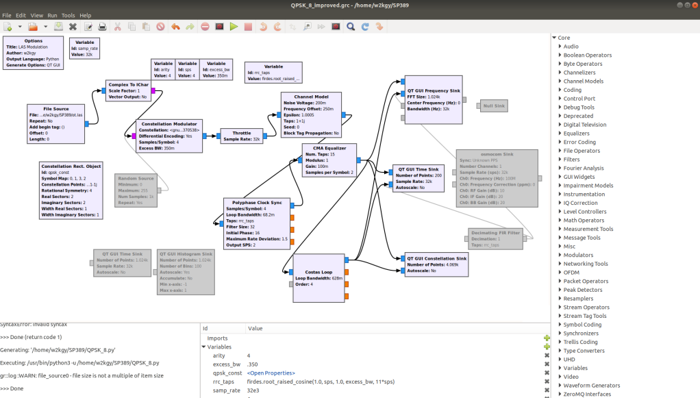
QPSK Flowgraph
Using the first 96 lines of LIDAR data resulted in the following display:

More Filtered QPSK
Comparison
For QPSK, I attached a BER block from the file sink and the receiver output to save to a central script. I did the same for QAM - QPSK had higher reception strength but QAM performed much quicker. Many satellites use QPSK for high data rate transfer, probably because of its improved BER. Both systems use the same bandwidth dependent on sampling as shown with the QPSK equation.
Extension: LoRa packets
Next, I am going to transmit my same LIDAR data using LoRa modules. The packet format of the LoRa devices ensure I have higher precision and error checking within my transmissions at the cost of higher bandwidth. I will try to use an Adafruit module aiding in my Commercial-Off-The-Shelf (COTS) angle. Hopefully this will show the reception strength of chirp spread spectrum packets.
Similarly, Hudson Valley Digital Network has a HASViolet LoRa module that I am looking to try out with LoRa and a sparkfun LIDAR sensor. I will keep you posted!
I also will be doing a deep dive into Amateur Television - another form of high-volume data transfer.
Lastly, I am going to fully flush out the experimentation of these modes. I plan on using a Step Attenuator to show the power threshold for each of my devices in a closed experimental environment.

Step Attenuator
Stay tuned!