Beamscanning DoA and Beamforming with MATLAB
In preparation for an upcoming project, I have been experimenting with the Phased Array Toolbox in MATLAB. I built a 10-antenna ULA and simulated some different forms of radio signals coming in. Enjoy!

Device Process and Theory
This device consists of two stages: Beamscanning and Beamforming. Beamscanning uses a phased array to give an estimate of azimuth for an incoming signal, while beamforming uses that azimuth estimation to optimize reception of the signal in question.
Beamscanning DoA
According to the MATLAB website, the beamscanning algorithm computes the output power for each beamscan angle and identifies the maxima as the DOA estimates. Beamscanning “sweeps” through the antenna array to determine the highest receive power. This gives it a relative azimuth estimate.

Visualization of a phased array
Beamforming
Beamforming is the second stage of this process. It acts in a similar, reverse manner - the phased array is “tuned” to maximize reception in the azimuth location given by the DoA estimation. This widely maximizes quality of signal reception. Beamforming can be transmit-or-receive, as the Beamforming term pertains to the antenna pattern from the phased array. In MATLAB, I used the “Phase-Delay” conventional beamformer found here.
Methods
For this experiment, I used a ULA of 10 isotropic antennas. For two tests, my signal had a carrier frequency of 150 MHz. The antennas were tuned specifically for this frequency. I kept the same angle for all three tests: 10 degrees azimuth and 20 degrees elevation. Although I did get similar results for the tests, there were actually wide discrepancies caused by the variation in modulation scheme.
Test 1: Square Wave
For the first test, I used MATLAB’s basic square() function. I gave it a frequency of about 300 Hz with the same carrier frequency of 150 MHz. This personally was not clear to me - the signal does not appear to be modulated in any way. Either way, it had great accuracy in estimating my angle of arrival - 10 degrees. It was off by 0.5 degrees with a percent error of 5%.

Square Wave Azimuth Estimation
Surprisingly, this wave was the only clear wave with this typical broadside angle spectrum.
The azimuth gain plot for the array proved its effictiveness:

Azimuth Plot for Square Wave
I did not note any significant difference in this plot for any of the tests, since my number of arrays were kept consistent. Lastly, one can see a clear reduction in noise while beamforming the square wave:
Beamformed Square Wave
Overall, the test was effective in maximizing receiver quality for the signal.
Test 2: ADS-B Signal
For an extension project down the line, I wanted to simulate ADS-B signals. I changed my carrier frequency to 1090 MHz and used a function to encode an ASD-B packet for a specified length of time. I kept the same azimuth and elevation, but got widely different results for the angle estimation:
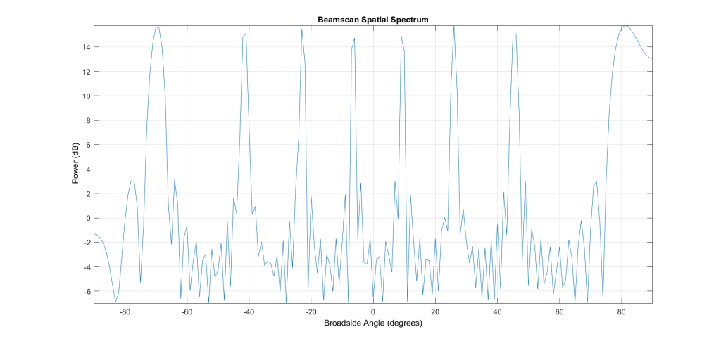
DoA for ADS-B
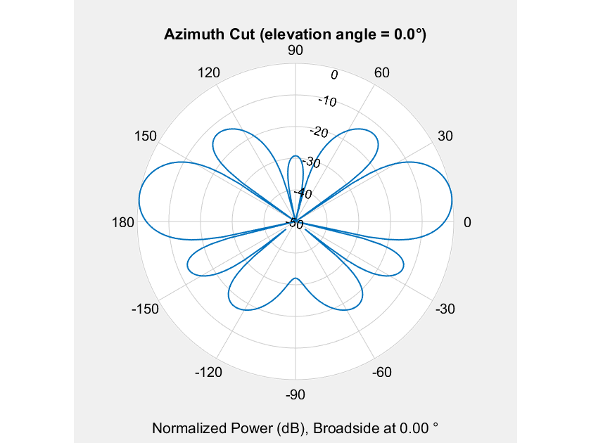
Nearly all the peaks are uniform spaced by 20 degrees. The “estimation output” function gave me 7 estimated arrival angles. This looks unsuccessful further echoed by the antenna gain plot:

Antenna Gain for 10-element ADS-B ULA
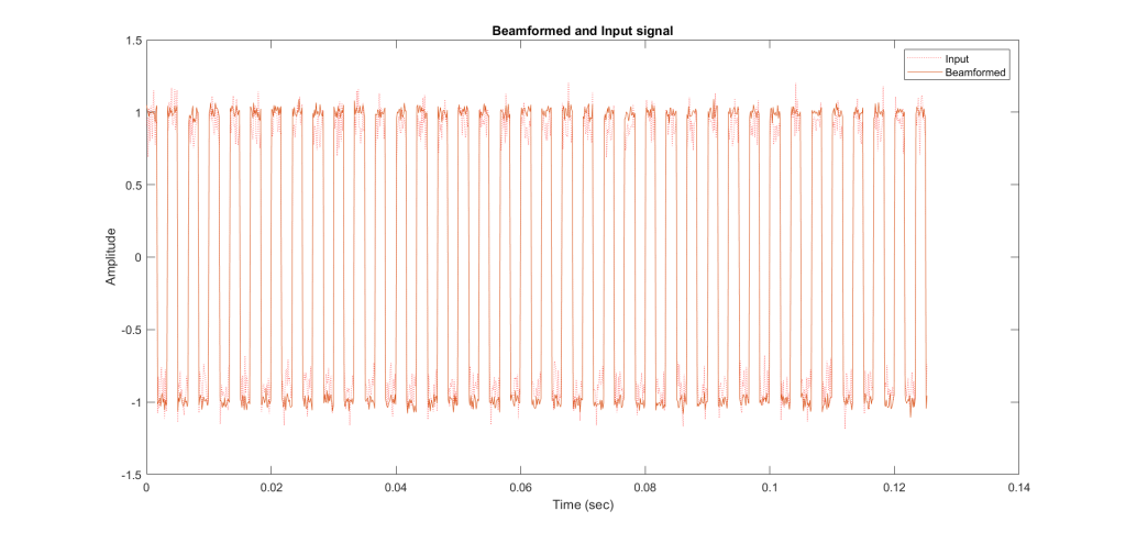
However, I did get mild improvement with the beamformed reception:

Beamformed ADS-B Signal
I will probably run this through a decoder to find the actual output. I imagine it will decode easier than the non-beamformed signal.
Test 3: AM Signal
For my final test, I took an audio file and AM modulated it on 150 MHz. My original audio is a voice recording of the word “beamforming” sampled at 8000Hz, available here. Just to make sure I modulated it correctly, I took the Fourier transform of my audio and the modulated signal. You can clearly see the double sidebands with the AM signal.

FFT for Am signal (blue) and Audio signal (orange)
The antenna array was able to estimate DoA much better than the previous two tests with no significant peaks away from the intended azimuth:

DoA Estimation for AM
This estimation and effectiveness is confirmed by the antenna’s azimuth gain plot:
Gain Plot for 10-element AM ULA
Finally, I was able to beamform and deconstruct the signal shown with the following plot:

Beamformed AM Signal
I was apprehensive that this signal was still a valid AM message and not just noise. After demodulating both signals, I did find the original message remained:

Lastly, after demodulating I recorded the outputs of the signal. The original received message (without beamforming) can be viewed here. This is unintelligible static, but the beamformed message results in slightly higher quality. One can almost hear “beamforming test” quickly compressed with background static.
Conclusion
Overall, a 10-element ULA was effective in locating the source of a square wave, ADS-B signal, and AM signal respectively. Using code provided here, I found the broadside angle plot, antenna gain plot, and reception visualization for all three tests. I found the highest accuracy with AM, and the lowest with ADS-B.
In the future, I will be constructing a beamforming phased array using coherent radio receivers. I cannot wait to update my results!