Magnetic Fields and Underwater Transmission Mediums
Hi again, I am working on modeling magnetic fields underwater. I came up with quite a few revelations and relationships, so I hope to present them in an easy-to understand way. Eventually, I want to combine these models and create a time-varying magnetic plane wave through a nonconductive medium such as water.
I’ve uploaded all my files here on github. I used mainly my electromagnetics textbook, Fundamentals of Applied Electromagnetics, 7th ed., by Fawwaz T. Ulaby and Umberto Ravaioli.
Simple Loop of Current
Pg. 247 gives an example of a magnetic field of a circular loop. This proves infinitely useful for any magnetic calculation, as loops often provide ample transmitting area and are easy to model B (magnetic flux density) and H (magnetic field intensity). I initially used the Biot-Savart law shown here:

Biot-Savart Law
Instead of dl, I took a surface integral of my surface - a flat copper ring. Here is a set up to my problem.
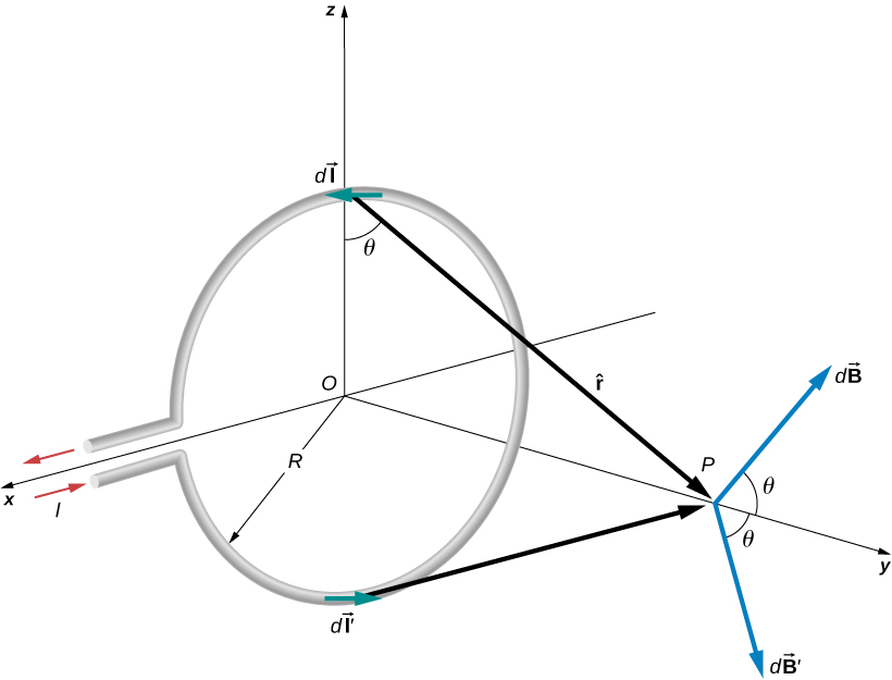
Current-Carrying Loop
After I took the two integrals (between 0 and 2 pi, and 0 and my radius in cylindrical coordinates), I got the result for magnetic field intensity from any distance directly on the center of the loop axis.:
H = I * a^2 / 2*(a^2 +z ^2)^3/2
Clearly, a 1/r3 relationship can be seen, with a similarly large role of the radius a.

The radius of the loop seemed to reach a peak value with a small diameter, which may be because of the input current or other values.

Mutual Inductance through 2 loops
I successfully modeled one loop, but now I have to measure two. I initially was going to model a transmitter and receive rig, but the equation turned too easy to model. In real-life application Helmholtz Coils are tuned to a specific resonance to enable a strong current with a uniform magnetic field. For two coils spaced two meters apart on the z axis, the resultant magnetic field intensity is:
= I*a^2 / 2 * (1/z^3 + 1/(z-2)^3)
If you are interested, look at page 276, figure 5.14. My equation made generalizing assumptions and was too simple for replication.

Standard Biot euqation through two loops.
However, for a TX and RX loop, mutual inductance can be defined as the energy stored in the magnetic field between these loops. Depending on the distance z, the mutual inductance represents a value in Henries dependent on number of turns, current, and separation distance.
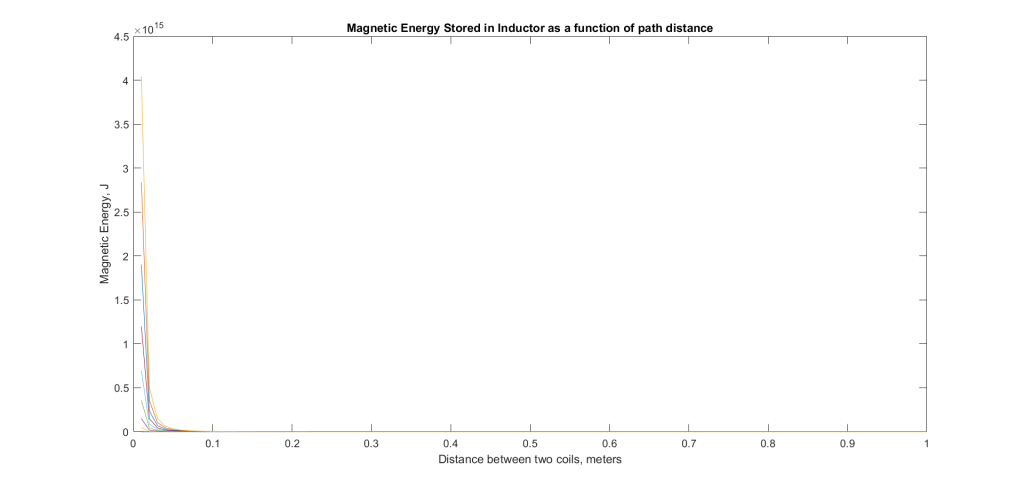
I multiplied this value L by the current I to get W, the magnetic energy stored in this system. It shows that there must be an incredibly small distance between the two coils at my radius for any energy storage.
Eventually I want to model this as a time-dependent relationship, since my energy is in Joules and not Watts.
Reflection Coefficient for Water
Due to our project, we have a high chance of interacting with air and water transmission mediums. In this study, I tried to replicate loss coefficients as a function of angle of incidence shown below. It is important to note that I have r as perpendicular and parallel; the parallel-polarized wave has a sharp decline near theta = 82. This value is the Brewster Angle, where the parallel-polarized wave is entirely transmitted by the second medium.
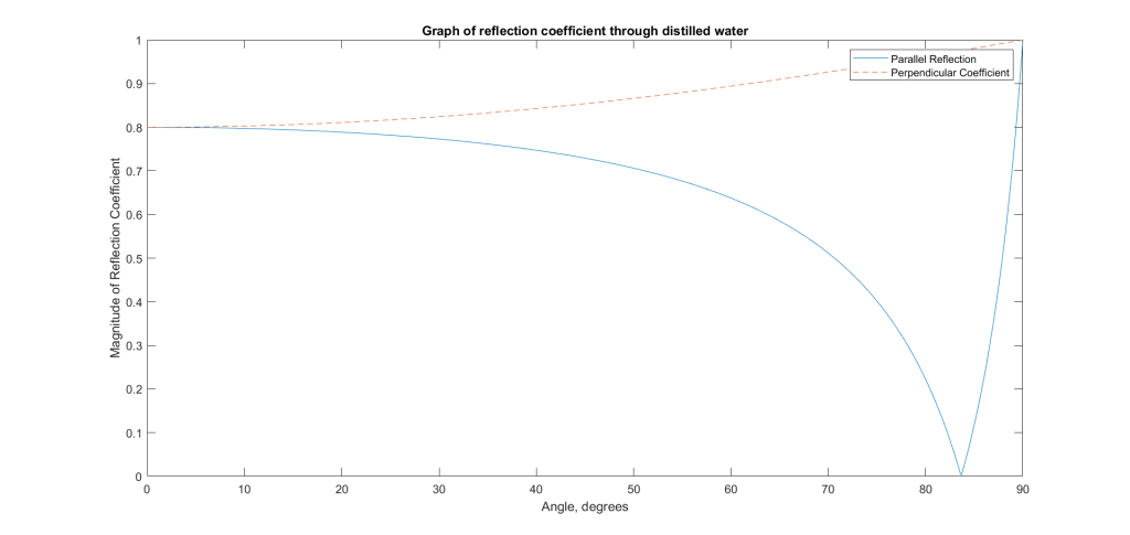
Reflection Coefficient Underwater
From this study, I can conclude that as the angle of transmission increases (to 90), the reflection constant decreases.
Time-Varying Field Underwater
Lastly, I brought several elements together and modeled a plane-wave underwater. When an electromagnetic wave transmits (like a radio) it transmits an electric field wave and my magnetic field wave. Its direction of propagation looks like this:

I was primarily concerned with the magnetic waves, as electric waves do not receive well under my constrained applications.
For my graph, I modeled an example for a H-field underwater using the textbook. It operates as a function of frequency (0 to 100 ohms_) and time(600ms)
Where n and m are unit steps for distance and time, respectively.H(n,m) = mag * exp(-.126*zz(n)) * cos(pi2e3tt(m) - .126*zz(n) + pi/12);

Upon closer look, the data follow a similar underdamped trend. I decided to improve upon the design with a matched 2d equation. This equation uses one variable, called mm, for all its calculation.
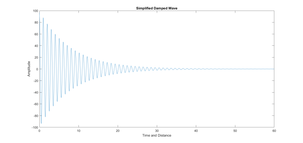
Simplified Damped equation,
Conclusions
This project was a fun dive back into my electromagnetics textbook. I was able to model several implementations of a magnetic field, wireless loop transmitter, and in the future I will combine them for a more cohesive equation.
Specifically with the plane wave assumptions there is a lot more to improve. I can attach a modulation scheme to the varying current and conduct a BER on the kHz required for operation. Magnetic loops tend to have low, predefined frequencies whose wavelength are several times larger than a transmitting distance.

Eventual goals shown with plane-wave propagation.
After those tests are concluded, I can attach a varying current and send data over magnetic loops!
This was an interesting project and I hope it continues to improve.