I’ve got a couple of ideas on my sketch pad that I needed to unload into a blog post. Here’s one I’m kicking around for a future date - a predictive model for a landing location of an amateur radio weather balloon.

Introduction

Statistics are powerful. Given enough data, we can make an informed decision on expectations and future events. This can be widely applied many fields - one being location estimation. If we’re given a sequence of positions, then we might just have enough information to make an prediction on the next location. But what information is necessary to make a comprehensive model? Not only do we need sufficient statistical information (a defined term meaning information about each of our variables, like position or velocity), but we need sufficient variables to give a good model. We could probably predict the position based on just the current position (more about that later), but more variables (like velocity, windspeed, altitude, even weather data) might give us a better prediction.

How do we test all this and see? There are other prediction resources, like habhub but I’m not looking to outperform these models just yet. Simulations will be our best bet here.

Also, habhub seems to be retiring in the near future. So other models may need to be used…

Method

This study lends itself to two scenarios:

Making a prediction before the launch occurs based on weather models and no data from the launch - “The forecast”
Making a live-updating prediction as the balloon is in the air, based on transmitted data - “The prediction”

Weather Modeling

I’m going to assume that weather models (windspeed especially) will give us a good indication of future balloon location. Weather models are an incredibly complex field, with little coherence or predictibility themselves. These models give us a forecast of weather at a specified point - useful if we don’t have the information ourselves. So what if we measure these parameters (windspeed, pressure, temperature), ourselves?

As an aside, the most accurate resource for weather prediction has been told to me as High Resolution Rapid Refresh. I’m not a climate scientist so I don’t know much about the model, but it will probably be useful for the forecast scenario.

Kalman Filter

Kalman Filters are often used for prediction modeling. They model a future state based on the past and current state. Broken down into position terms, it has the capability to estimate the future position based on past and current position - seems quite useful. Plenty of websites offer a better explanation, but I’ll write it here for my own sake:

I’m going to take directly from this website as it has a straightforward approach I’ve seen on other websites:

Simple Position Estimation

Take this 1-d position equation:

$ x = x_0 + v_0 \Delta t + \frac{1}{2} a \Delta t^2 $

Where:

$x$ is the position
$x_0$ is the initial position
$v_0$ is the initial velocity
$a$ is the acceleration
$\Delta t$ is the time interval

This can be applied to three dimensions as well, but I’ll keep it in 1D to avoid overcomplicating.

The variables (parameters) $[x,v,a]$ make the System State. The current state is the input to the prediction, and the following state is the output. This means, of our two scenarios, the prediction scenario can “easily” predict the next state.

However, random error is introduced in this equation. We have weather aspects and the balloon isn’t moving in a straight line. There is both Measurement Noise and Process Noise that increase error and disrupt our otherwise perfect estimation.

The Kalman filter uses these noise considerations to improve prediction.

For more statistics removed from our application, go to the Second Page of Alex Becker’s explanation.

State Update

Let’s say our position isn’t changing, but we are still getting variation for each measurement. Obviously this will be a little less difficult than estimating a moving position, so we don’t need as much information or processing time.

Generally to find the average position we can just take the average:

$\hat{x}_{n,n} = \frac{1}{n} \Sigma{i=1}^n (z_i)$

Here, $\hat{x}_{n,n}$ is our estimation, $n$ is the index of measurement, and $z_i$ is the measurement.

The next position will probably depend more on its most recent position than its long-past positions, right? After some more derivation (available here), we get:

$\hat{x}{n,n} = \hat{x}{n,n-1} + \frac{1}{n} (z_n - \hat{x}_{n,n-1})$

Which shows the estimation at state $n-1$ is based on the measurement at $n$. In english terms:

StateUpdate

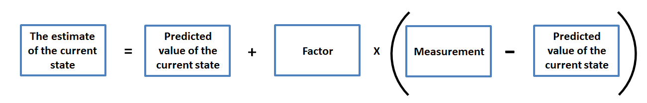
That $\frac{1}{n}$ is important. It is the Kalman Gain, $K_n$, and changes as $n$ changes. It is the “factor” from the image above, and specific to our example. If we increase n (more measurements or time), then the $(z_n - \hat{x}_{n,n-1})$ term will have a smaller weight.

This equation also relies on an initial guess, which may be difficult for a turbulent balloon.

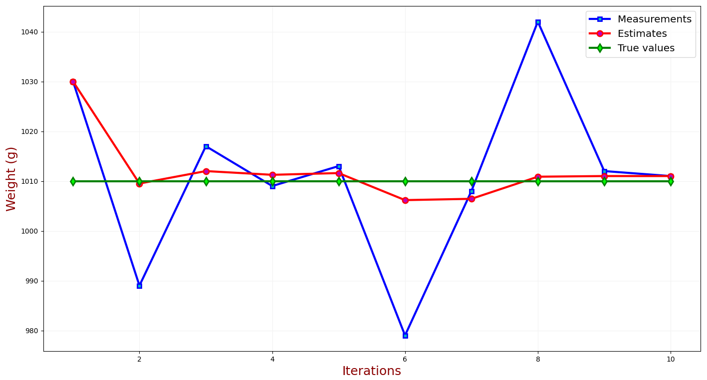
Becker finishes this example with a simulation where he guesses the weight of a gold bar after several iterations. As the iterations increaes, the error decreases and the estimate approaches the true value:

Estimation

Position and Velocity Equations

Becker gives two equations for position and velocity based on the state update equation and constants $\alpha$ and $\beta$:

Position:

$\hat{x}{n,n} = \hat{x}{n,n-1} + \alpha (z_n - \hat{x}_{n,n-1})$

Velocity ($\hat{\dot{x}}_{n,n} = v$, the derivative of position)

$\hat{\dot{x}}{n,n} = \hat{\dot{x}}{n,n} + \beta (\frac{z_n - \hat{x}_{n,n-1}}{\Delta t})$

The values for $\alpha$ and $\beta$ depend on the ability of the measuring software. Becker explains that high-performace equipment results in a high $\alpha$ and $\beta$, almost as a “faith factor.”

This is then expanded to acceleration and uncertainty.

Statistical Estimation

Nothing was particularly interesting about our derivations for the estimation. It all depended determininstically on the past states. But, we can assume that the measurements for position are going to change, and that they will change following some form of distribution.

This is where the magic happens. We want to minimize the error between our estimation and the true value, so we can use forms of estimation like Minimum-Mean Squared Error or Minimum Variance Ubbasied Estimation.

Becker uses these relationships to define a better equation for the Kalman Gain $K_n$:

$K_n = \frac{\text{Uncertainty in Estimate}}{\text{Uncertainty in Estimate+ Uncertainty in Measurement}}$

He determines the uncertainty in the estimation as:

$p_{n,n} = (1-K_n) p_{n,n-1}$

This results in 5 equations called the Kalman filter Equations.

Noise

GPS measurements are not exact - they introduce small imprecisions. Even though we are looking to estimate the true position, even the GPS doesn’t know what the true position is. We need the variance $\sigma^2$ to assist in estimation. We estimate this variance, and get a resulting Estimate Uncertainty.

This depends on Process Noise, and process noise has its own weight - some processes, like temperature measurement, may have a low noise because it only depends on the variance of a thermometer. However, position estimation (and especially turbulent balloon estimation) will have a very high process noise.

Matricies and Multiple dimensions

I’m still following along with Becker’s Website adding my own knowledge where I see fit. He describes some relationships between multiple variables such as covariance and variance.

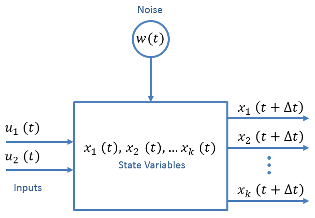
He presents a general matrix equation for the state equation:

$\boldsymbol{\hat{x}{n+1,n}} = \boldsymbol{F \hat{x{n,n}}} + \boldsymbol{G u_n} + \boldsymbol{w_n}$

This is all very exciting. Definitions:

$\boldsymbol{\hat{x}_{n+1,n}}$ is the prediction of the future state (like future position)
$\boldsymbol{\hat{x}_{n,n}}$ is the current prediction
$\boldsymbol{u_n}$ is a control variable - like windspeed or pressure
$\boldsymbol{w_n}$ is the noise that affects the measurement
$\boldsymbol{F}$ is the state transmition matrix
$\boldsymbol{G}$ is the control matrix, mapping the control variables to the state variables.

Nicely put in a block diagram:

This equation is used for many kalman filtering problems, and is explained in application via matlab

I’m going to put a pin in this section as I continue to read and understand Kalman filters. Still follow along with Becker as he does a good job explaining matrix applications and derivations for the kalman equations.

Experimental Setup

So if I were to build this model equation, I’d need the information I am estimating (position), control variables, and measurement equations that transform these control variables.

Parameters to record

Measurement variables:

GPS Position
Velocity
Acceleration (noise will be introduced at each of these stages)
Wind Speed and direction
Altitude

Parameters from models

It would be interesting to investigate, but I wonder if the pressure or humidity in the upper atmosphere changes prediction. Similiarly, some parameters of the balloon that concern wind (weight, surface area) are non-changing but may drastically increase or decrease acceleration.

Control variables:

Payload Weight
Payload surface area
Lift calculations from hydrogen

Partslist

If I were to build a payload that would measure the variables I want:

High-Altitude GPS Receiver
Accelerometer
Anemometer (something like this)
Wind vane (reed switch as a possibility)
Gyrometer to account for wind direction measurement

Experimental Goal

I’d have to transmit all the recorded parameters over radio to a downlink for prediction. or I could run predictions about the balloon and tramsit the prediction down, but that introduces too many opportunities to go awry.

This may require an APRS transmitter using the telemetry mode to use the 12 available fields for the parameter information. I’ve done some work with APRS transmitters so this isn’t out of the wheelhouse for me - it may be a design similiar to the Microtrak but with programmable telemetry fields.

Next Steps

This has really tickled me as a fun experiement and prediction scenario. I’ll update it in the future if I get anywhere with the prediction software or board design.