More DSP Applications in MATLAB

Back again with the rest of my findings on DSP in matlab. I dove deep into DTMF encoding, AM signals, and some image processing. I used the textbook DSP First for most of these examples. In some of these examples, I relied on external functions found in the SPFirst Toolbox.

Amplitude Modulation

DTMF Encoding

DTMF, Dual-Tone Multi Frequency Signaling, operates on a grid system. Each digit corresponds to two different tones.

In Matlab, you can use two separate row vectors (or probably a matrix if you’re smarter than I am) that corresponds to the tone. The encoder I made (here) simply takes an array of numbers (like a phone number), then finds each tone. It uses the sound() function to play each tone sequentially.

In the future I will make a decoder as well as an encoder, and probably improve my design.

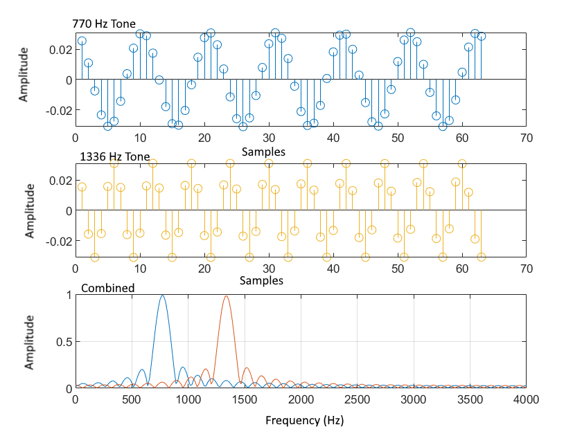
Discrete representation of two DTMF tones, and their combined frequency response

AM Mixing and Filtering

I had a lot of fun with this one. AM Signals have a message signal and a carrier signal inside each other. The resultant signal is a function of both previous signals. With the help of a filter, you can decode AM signals to get your original message signal back again. This of course is nothing new, as it’s how every AM radio works. But it is super interesting to see it visualized. My encoding/decoding script is again on github.

My message and carrier signals can be written as the following sinusoids:

mm = A*cos(2*pi*fm*nn);
cc = cos(2*pi*fc*nn);
xx = (1+mm).*cc;

Where fm is the message frequency, fc is the carrier frequency, and nn is a time-independent sequence.

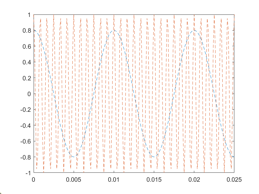
Here’s the message signal (blue) with the carrier signal (orange)

When you filter the AM signal, you are trying to remove the orange. This can be done with the matlab function firfilt which uses coefficients in an array b. You can keep filtering the resulting array on itself for greater effects.

bb = [1, 0, 1];
yy = firfilt(bb, xx);

Here it is as a function of frequency. The original signal is purple, and the filtered signals in blue and orange.

So the frequency in a time domain looks like this:

The solid orange line is the original message. Not sure about the solid horizontal line…

So if you run through the whole process, you can create a message, encode it, then decode it. Sort of like playing catch with yourself. Here’s my version.

Image Processing and Filtering

I had a lot of fun with this one. Instead of one sinusoid, you create a column of 256 of them! This is the basis of image processing. Below, I set up my frequency and graphed the result. This is a result of grayscale, where every pixel is a shade of gray between 0 and 255. Link

tt = 1:256;
yy = sin(2*pi/50*tt);
a = ones(256,256);
a = a.*yy;

The resulting image:

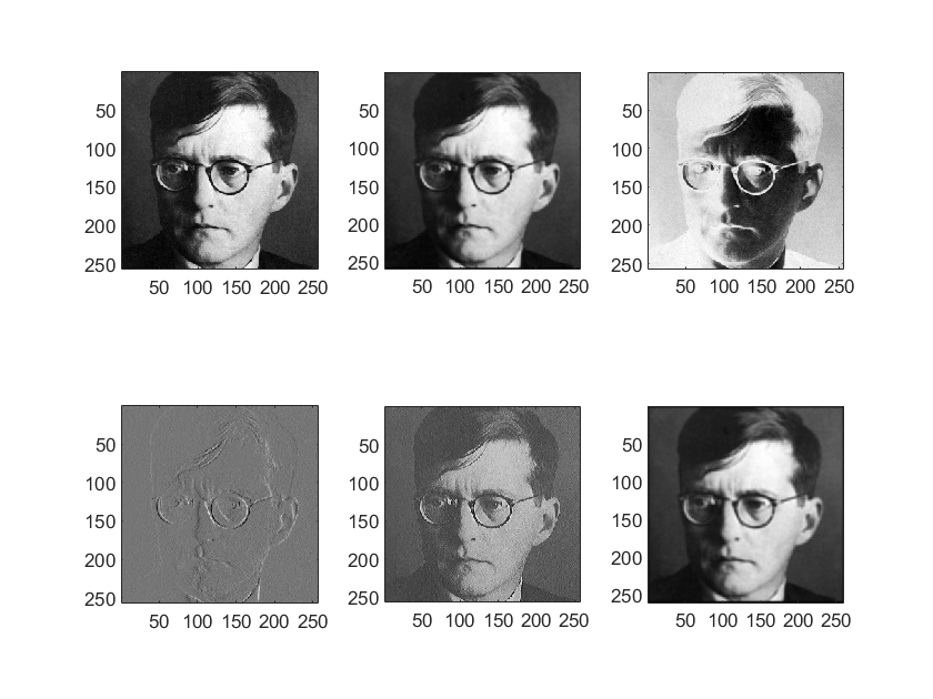
Next, I did some manipulation of 256 x 256 images in grayscale.

I used the firfilt() both horizontally and vertically to blur the image. Here is what it looks like standard, horizontally blurred, vertically blurred, and blurred on both dimensions.

Eyesight fading

From here I experimented with different coefficient values for the FIR filter. Some will produce a high-passs filter instead of a low-pass. This means you will have some unique turn outs:

Lastly, I made a negative() function to return the negative of the image. Code:

 img = img ./ 256;
 img = 1- img;
 negativeimg = img .* 256;

Where each grayscale value is normalized, subtracted from 1, and returned to grayscale format. In total you get this nice Warhol-looking Shostakovich art:

There’s a lot more I have yet to do with image filtering and processing.

Closing

MATLAB has tons of cool ways to create manipulate, and interpret digital signals. While I have to break the surface still on Fourier Transforms, I had a lot of fun messing with these signals.